Alignment Visualization - IGV
Now that our BAM files have been indexed with samtools we can load them and explore the RNA-seq alignments using the Integrative Genomics Viewer (IGV).
The exercise below assumes that you have IGV installed on your local computer. If you are unable to get IGV to run locally you may also consider a web based version of IGV that runs in your browser. The interface of the IGV Web App is different from the local install, and is missing a few features, but is conceptually very similar. To access it simply visit: IGV Web App.
Visualize alignments with IGV
Start IGV on your computer/laptop. Load the UHR.bam & HBR.bam files in IGV. If you’re using AWS, you can load the necessary files in IGV directly from your web accessible amazon workspace (see below) using ‘File’ -> ‘Load from URL’.
Make sure you select the appropriate reference genome build in IGV (top left corner of IGV): in this case hg38.
AWS links to bam files
-
UHR hisat2 alignment: http://YOUR_PUBLIC_IPv4_ADDRESS/rnaseq/alignments/hisat2/UHR.bam
-
HBR hisat2 alignment: http://YOUR_PUBLIC_IPv4_ADDRESS/rnaseq/alignments/hisat2/HBR.bam
Links to cached version of these bam files
If for some reason you do not have access to the BAM files from running through this course you can download and use these cached versions instead:
You may wish to customize the track names as you load them in to keep them straight. Do this by right-clicking on the alignment track and choosing ‘Rename Track’.
Go to an example gene locus on chr22:
- e.g. EIF3L, NDUFA6, and RBX1 have nice coverage
- e.g. SULT4A1 and GTSE1 are differentially expressed. Are they up-regulated or down-regulated in the brain (HBR) compared to cancer cell lines (UHR)?
- Mouse over some reads and use the read group (RG) flag to determine which replicate the reads come from. What other details can you learn about each read and its alignment to the reference genome.
Exercise
Try to find a variant position in the RNAseq data:
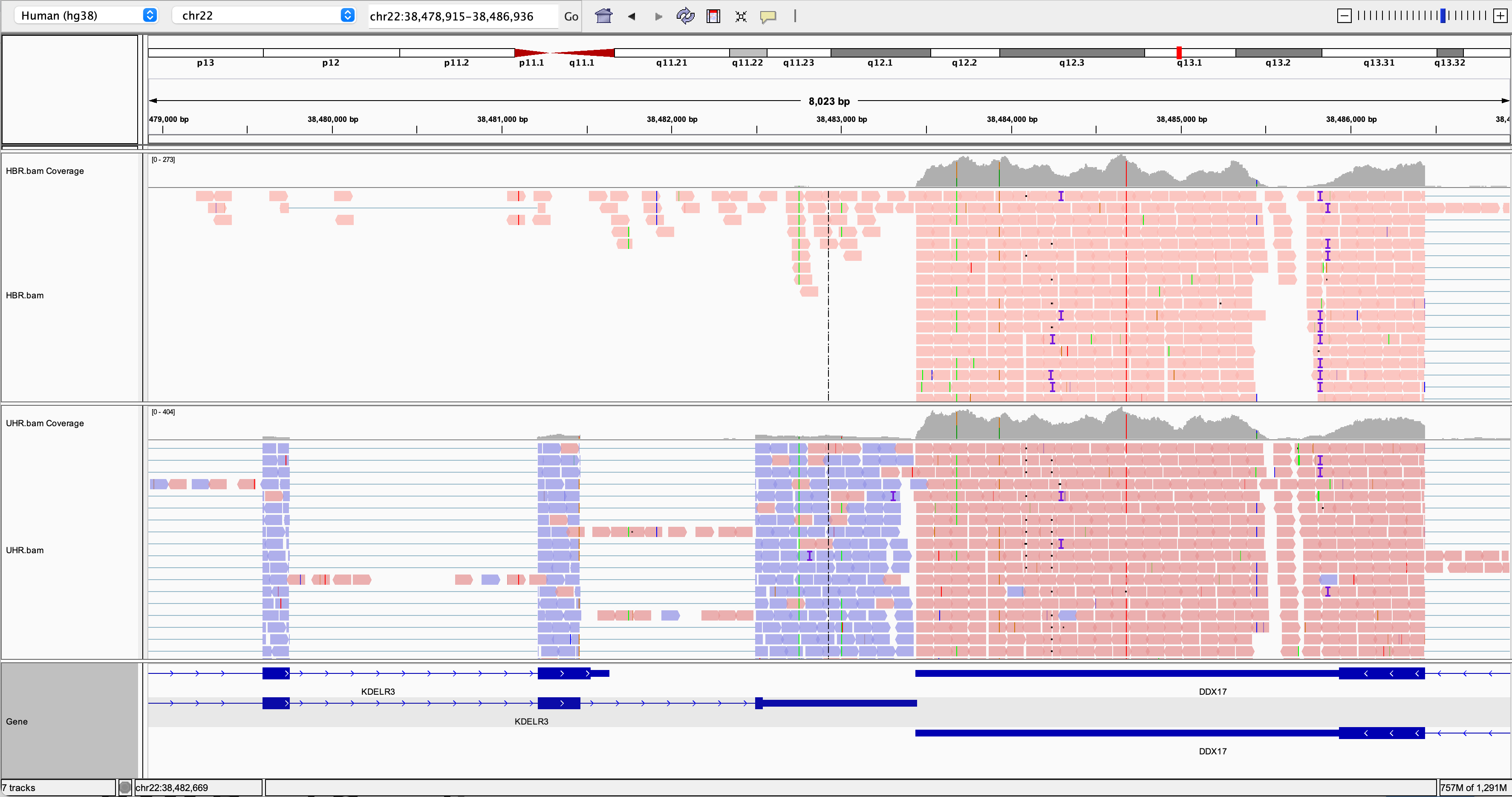
- HINT: DDX17 is a highly expressed gene with several variants in its 3 prime UTR.
- Other highly expressed genes you might explore are: NUP50, CYB5R3, and EIF3L (all have at least one transcribed variant).
- Are these variants previously known (e.g., present in dbSNP)?
- How should we interpret the allele frequency of each variant? Remember that we have rather unusual samples here in that they are actually pooled RNAs corresponding to multiple individuals (genotypes).
- Take note of the genomic position of your variant. We will need this later.
IGV visualization example (DDX17 3 prime region)
PRACTICAL EXERCISE 7
Assignment: Index your bam files from Practical Exercise 6 and visualize in IGV.
- Hint: As before, it may be simplest to just index and visualize the combined/merged bam files HCC1395_normal.bam and HCC1395_tumor.bam.
- If this works, you should have two BAM files that can be loaded into IGV from the following location on your cloud instance:
- http://YOUR_PUBLIC_IPv4_ADDRESS/rnaseq/practice/alignments/hisat2/
Links to cached version of the practical exercise bam files
If for some reason you do not have access to the BAM files from running through this course you can download and use these cached versions instead:
Questions
- Load your merged normal and tumor BAM files into IGV. Navigate to this location on chromosome 22: ‘chr22:38,466,394-38,508,115’. What do you see here? How would you describe the direction of transcription for the two genes? Does the reported strand for the reads aligned to each of these genes appear to make sense? How do you modify IGV settings to see the strand clearly?
- How can we modify IGV to color reads by Read Group? How many read groups are there for each sample (tumor & normal)? What are your read group names for the tumor sample?
- What are the options for visualizing splicing or alternative splicing patterns in IGV? Navigate to this location on chromosome 22: ‘chr22:40,363,200-40,367,500’. What splicing event do you see?
Solution: When you are ready you can check your approach against the Solutions.