Posts
My thoughts and ideas
Welcome to the blog
My thoughts and ideas
Introduction to bioinformatics for RNA sequence analysis
Single-cell sequencing gives us a snapshot of what a population of cells is doing. This means we should see many different cells in many different phases of a cell’s lifecycle. We use trajectory analysis to place our cells on a continuous ‘timeline’ based on expression data. The timeline does not have to mean that the cells are ordered from oldest to youngest (although many analysis uses trajectory to quantify developmental time). Generally, tools will create this timeline by finding paths through cellular space that minimize the transcriptional changes between neighboring cells. So for every cell, an algorithm asks the question: what cell or cells is/are most similar to the current cell we are looking at? Unlike clustering, which aims to group cells by what type they are, trajectory analysis aims to order the continuous changes associated with the cell processes.
The metric we use for assigning positions is called pseudotime. Pseudotime is an abstract unit of progress through a dynamic process. When we base our trajectory analysis on the transcriptomic profile of a cell, less mature cells are assigned smaller pseudotimes, and more mature cells are assigned larger pseudotimes.
Earlier we confirmed that our epithelial cell population corresponded to our tumor population. Then, through differential expression analysis, we saw that the epithelial cells form two distinct clusters that we identified as luminal and basal cells. We can further confirm this conclusion by using trajectory analysis to assign pseudotime values to the epithelial cells. We expect see that basal cells are less differentiated than luminal cells.
First, let’s load our libraries and our preprocessed object.
library(Seurat)
library(CytoTRACE)
library(monocle3)
library(ggplot2)


merged <- readRDS('outdir_single_cell_rna/preprocessed_object.rds')
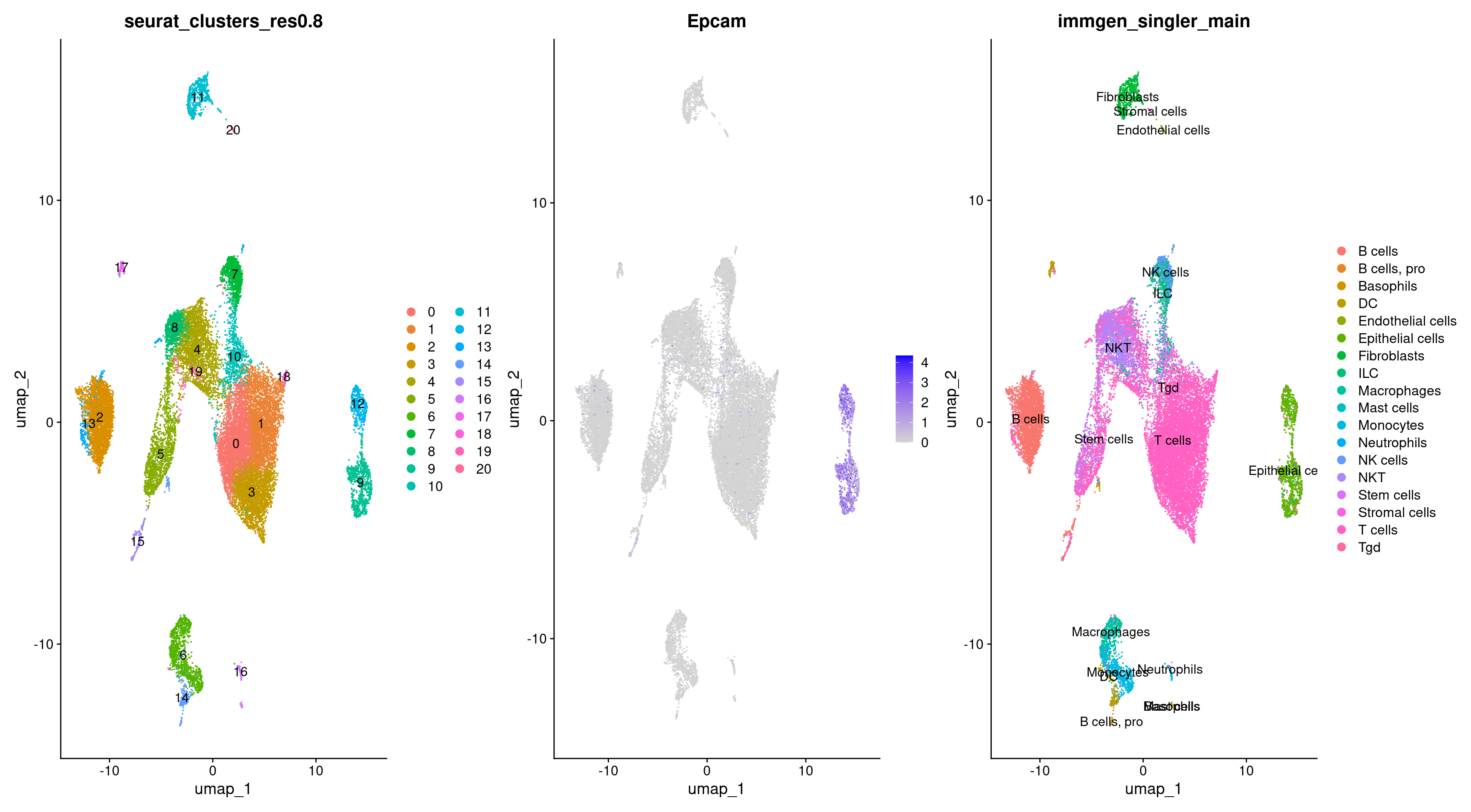
Let’s see what clusters our epithelial cells are located in.
DimPlot(merged, group.by = 'immgen_singler_main', label = TRUE) +
  DimPlot(merged, group.by = 'seurat_clusters_res0.8', label = TRUE)
We can specifically highlight these cells for further clarity.
Epithelial_cells = merged$immgen_singler_main =="Epithelial cells"
highlighted_cells <- WhichCells(merged, expression = immgen_singler_main =="Epithelial cells")
DimPlot(merged, reduction = 'umap', group.by = 'orig.ident', cells.highlight = highlighted_cells)
We already know that these two clusters can be separated into basal and luminal cells. We can see the distinction between these two types using markers. For example lets plot basal cell markers:
FeaturePlot(object = merged, features = c("Cd44", "Krt14", "Krt5", "Krt16", "Krt6a"))
To more comprehensively see where the basal and luminal cells are, we can create a cell type score by averaging the expression of a group of genes and ploting the score.
cell_type_Basal_marker_gene_list <- list(c("Cd44", "Krt14", "Krt5", "Krt16", "Krt6a"))
merged <- AddModuleScore(object = merged, features = cell_type_Basal_marker_gene_list, name = "cell_type_Basal_score")
FeaturePlot(object = merged, features = "cell_type_Basal_score1")

cell_type_Luminal_marker_gene_list <- list(c("Cd24a", "Erbb2", "Erbb3", "Foxa1", "Gata3", "Gpx2", "Krt18", "Krt19", "Krt7", "Krt8", "Upk1a"))
merged <- AddModuleScore(object = merged, features = cell_type_Luminal_marker_gene_list, name = "cell_type_Luminal_score")
FeaturePlot(object = merged, features = "cell_type_Luminal_score1")
For ease and clarity, let’s subset our Seurat object to just the epithelial cell clusters.
### Subsetting dataset epithelial
merged <- SetIdent(merged, value = 'seurat_clusters_res0.8')
merged_epithelial <- subset(merged, idents = c('9', '12')) # 1750

#confirm that we have subset the object as expected visually using a UMAP
DimPlot(merged, group.by = 'seurat_clusters_res0.8', label = TRUE) +
  DimPlot(merged_epithelial, group.by = 'seurat_clusters_res0.8', label = TRUE)

#confirm that we have subset the object as expected by looking at the individual cell counts
table(merged$seurat_clusters_res0.8)
table(merged_epithelial$seurat_clusters_res0.8)
Now let’s run CytoTRACE. CytoTRACE (Cellular (Cyto) Trajectory Reconstruction Analysis using gene counts and Expression) is a computational method that predicts the differentiation state of cells from single-cell RNA-sequencing data. CytoTRACE uses gene count signatures (GCS), or the correlation between gene count and gene expression levels to capture differentiation states.
# create a dataframe of expression values to pass to Cytotrce
merged_epithelial_expression <- data.frame(GetAssayData(object = merged_epithelial, layer = "data"))

merged_epithelial_cytotrace_scores <- CytoTRACE(merged_epithelial_expression, ncores = 1)
We then have to get the Cytotrace data into the correct format.
merged_epithelial_cytotrace_transposed <- as.data.frame(merged_epithelial_cytotrace_scores$CytoTRACE)
names(merged_epithelial_cytotrace_transposed) <- "cytotrace_scores"

head(merged_epithelial_cytotrace_transposed)

# fix the barcode formatting
rownames(merged_epithelial_cytotrace_transposed) <- sub("\\.", "-", rownames(merged_epithelial_cytotrace_transposed))
rownames(merged_epithelial_cytotrace_transposed)
Add the data to the object
merged_epithelial <- AddMetaData(merged_epithelial, merged_epithelial_cytotrace_transposed, 'cytotrace_scores')
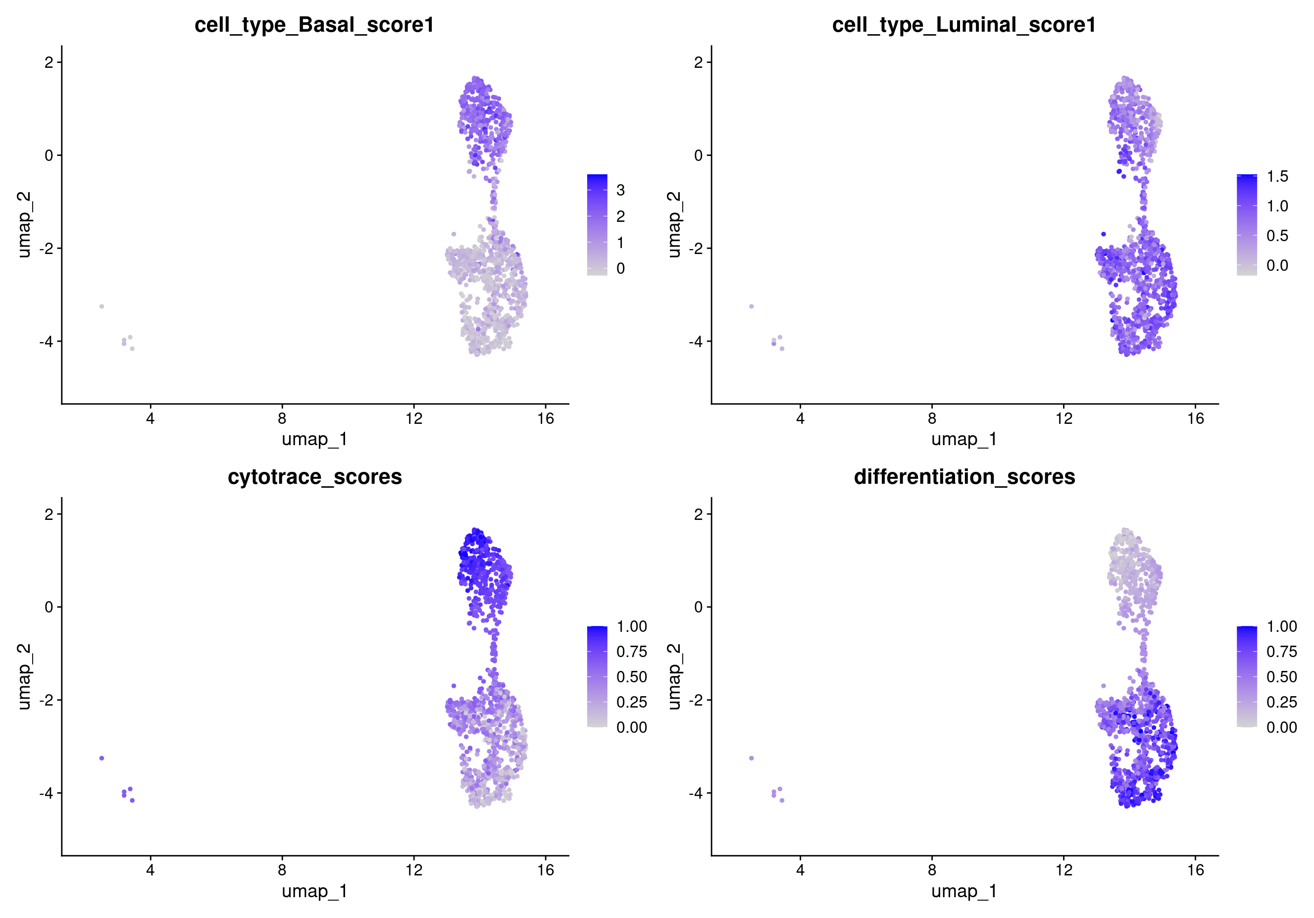
merged_epithelial[['differentiation_scores']] <- 1 - merged_epithelial[['cytotrace_scores']] # Let's also reverse out CytoTRACE scores so that high means more differentiated and low means less differentiated
FeaturePlot(object = merged_epithelial, features = c("cell_type_Basal_score1", "cell_type_Luminal_score1", "cytotrace_scores", "differentiation_scores"))
The most important part of trajectory analysis is to make sure you have some biological reasoning to back up the pseudotime values. The best practice for pseudotime means using it to support a biological pattern that has already been observed by some other method.
Let’s separate our luminal cells from the basal cells and perform trajectory analysis.
## Subset to just luminal cells
DimPlot(merged_epithelial) # cluster 10 is our luminal cells
merged_luminal <- subset(merged_epithelial, idents = c('9')) # 863 cells
We can also use the CytoTRACE R package to calculate our CytoTRACE scores.
# Creating a dataframe to pass to CytoTRACE
merged_luminal_expression <- data.frame(GetAssayData(object = merged_luminal, layer = "data"))

merged_luminal_cytotrace_scores <- CytoTRACE(merged_luminal_expression, ncores = 1)

merged_luminal_cytotrace_transposed <- as.data.frame(merged_luminal_cytotrace_scores$CytoTRACE)
names(merged_luminal_cytotrace_transposed) <- "cytotrace_scores"

head(merged_luminal_cytotrace_transposed)

# fix the barcode formatting
rownames(merged_luminal_cytotrace_transposed) <- sub("\\.", "-", rownames(merged_luminal_cytotrace_transposed))
rownames(merged_luminal_cytotrace_transposed)
We then can add those CytoTRACE scores to our luminal cell object and visualize them.
merged_luminal <- AddMetaData(merged_luminal, merged_luminal_cytotrace_transposed)
merged_luminal[['cytotrace_scores_luminal']] <- 1 - merged_luminal[['cytotrace_scores']]
merged_luminal[['differentiation_scores_luminal']] <- 1 - merged_luminal[['differentiation_scores']]
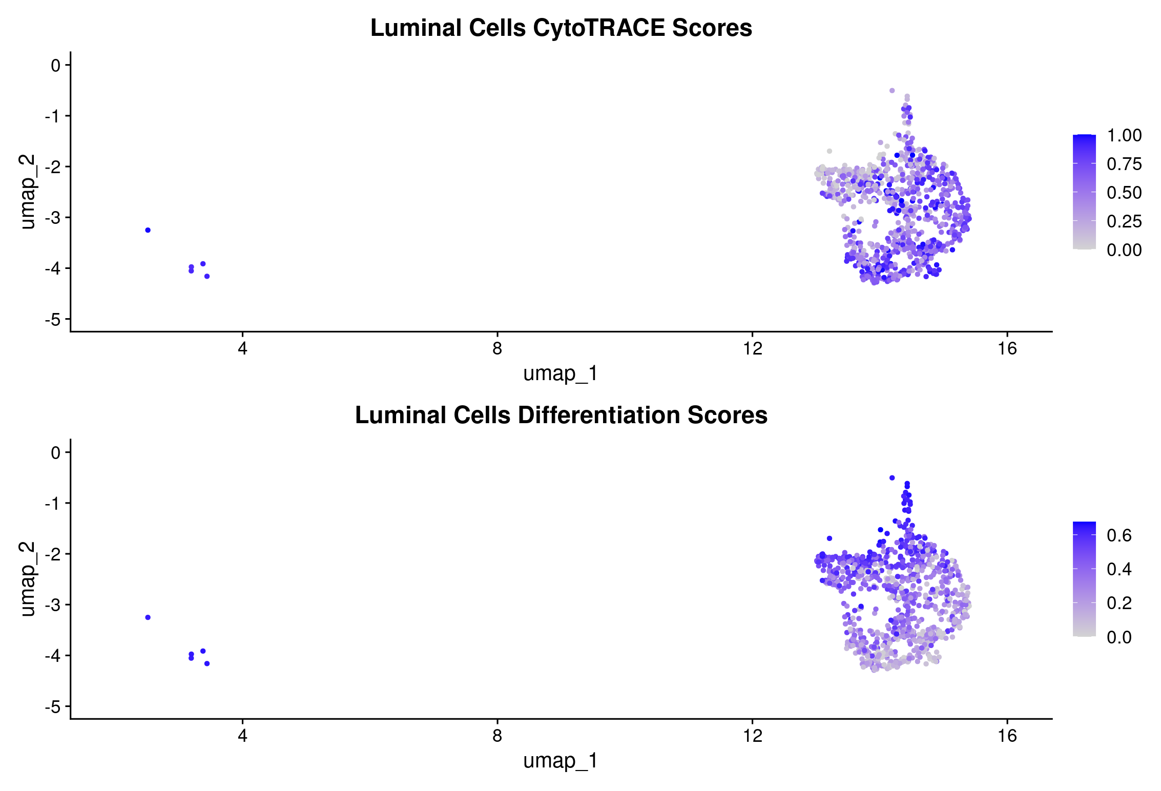
# compare all epithelial cells CytoTRACE scores to the luminal-only CytoTRACE
(FeaturePlot(object = merged_luminal, features = c("cytotrace_scores_luminal")) +
ggtitle("Luminal Cells CytoTRACE Scores")) +
(FeaturePlot(object = merged_luminal, features = c("differentiation_scores_luminal")) +
ggtitle("Luminal Cells Differentiation Scores"))
CytoTRACE will force all given cells onto the same scale meaning that there has to be cells at both the low and high ends of differentiation. The CytoTRACE scores could be a reflection of cell cycling genes. We can check by using a feature plot to compare the S-phase genes, G2/M-phase genes, and differentiation scores.
# View the S-phase genes, G2/M-phase genes, and the Phase to see if that explains the differentiation score
FeaturePlot(object = merged_luminal, features = c("S.Score", "G2M.Score")) +
   DimPlot(merged_luminal, group.by = "Phase")

FeaturePlot(object = merged_luminal, features = c("S.Score", "G2M.Score", "differentiation_scores"))
We still don’t see a clear pattern, which illustrates the challenge and the danger of pseudotime.
Exercise: Create a subset of the Seurat object. You could explore the differences between the T-Cells populations, stem cells vs epithelial cells, or choose your own subset. Then run CytoTRACE on the subsetted dataset either using the webtool or the R package. Do the pseudotime scores make sense? Are there biological factors that support the CytoTRACE calculated trajectory?
Note: CytoTRACE will crash in the posit environment if you give it too many cells, so if there are several cell populations that you want to compare you can use the subset function to downsample your cell types. Make sure your Idents are set to the category you would like to subset too!
merged_subset <- subset(x = merged, downsample = 100)
Now that we have convinced ourselves that we somewhat trust the results of CytoTRACE, we can try the algorithms on the entire dataset and compare it to another trajectory analysis method. Another popular method used is Monocle3. Monocle3 is an analysis toolkit for scRNA and has many of the functions that Seurat has. We can use Monocle3’s trajectory algorithm but since it uses its own unique data structure, we will have to convert our subsetted object to a cell data set object. Luckily, there are tools that make that conversion relatively easy.
You can also refer to the full Monocle3 trajectory tutorial.
Before we start just running our data through the algorithm and seeing what we get, we should consider what we expect to get. Let’s remember what cell types we have in our dataset and where they are on our UMAP. What pseudotime scores do you expect to be assigned to the clusters?
DimPlot(merged, group.by = 'immgen_singler_main', label = TRUE)
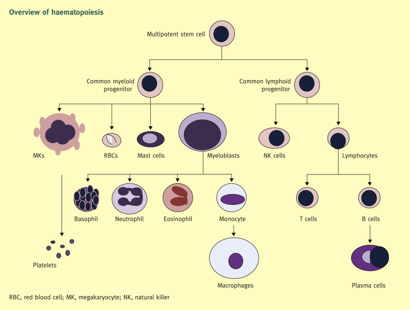
Haematopoiesis and red blood cells
Let’s now run Monocle3, again we have to convert our Seurat object to a Monocle ‘Cell Data Set’. We will use a package made for this specific purpose.
merged_cds <- SeuratWrappers::as.cell_data_set(merged)
Then we run the Monocle function cluster_cells. This function will redo unsupervised clusters and calculate partitions which are groups of cells that Monocle3 puts on separate trajectories. We don’t need the cells to be clustered since we already did that in Seurat but Monocle requires that partitions be calculated for its trajectory functions.
merged_cds <- cluster_cells(merged_cds)
Use the Monolce3 plotting functions to visualize partitions. Then we will execute the function learn_graph which will build the trajectory. We will set the use_partition parameter to FALSE so that we learn a trajectory across all clusters. Later you can come back and try setting it to TRUE and see what happens!
plot_cells(merged_cds, show_trajectory_graph = FALSE, color_cells_by = "partition")

# Monocle will create a trajectory for each partition, but we want all our clusters
# to be on the same trajectory so we will set `use_partition` to FALSE when
# we learn_graph

merged_cds <- learn_graph(merged_cds, use_partition = FALSE) # graph learned across all partitions
Monocle3 requires you to choose a starting point or root for the calculated trajectories. Running the function order_cells will open a pop-up window where you can interactively choose where you want your roots to be. Note that you have to allow pop-ups for this function because it opens a window to choose the roots in, your browser might have this disabled.
merged_cds <- order_cells(merged_cds)
# Pick a root or multiple roots
Plot the pseudotime:
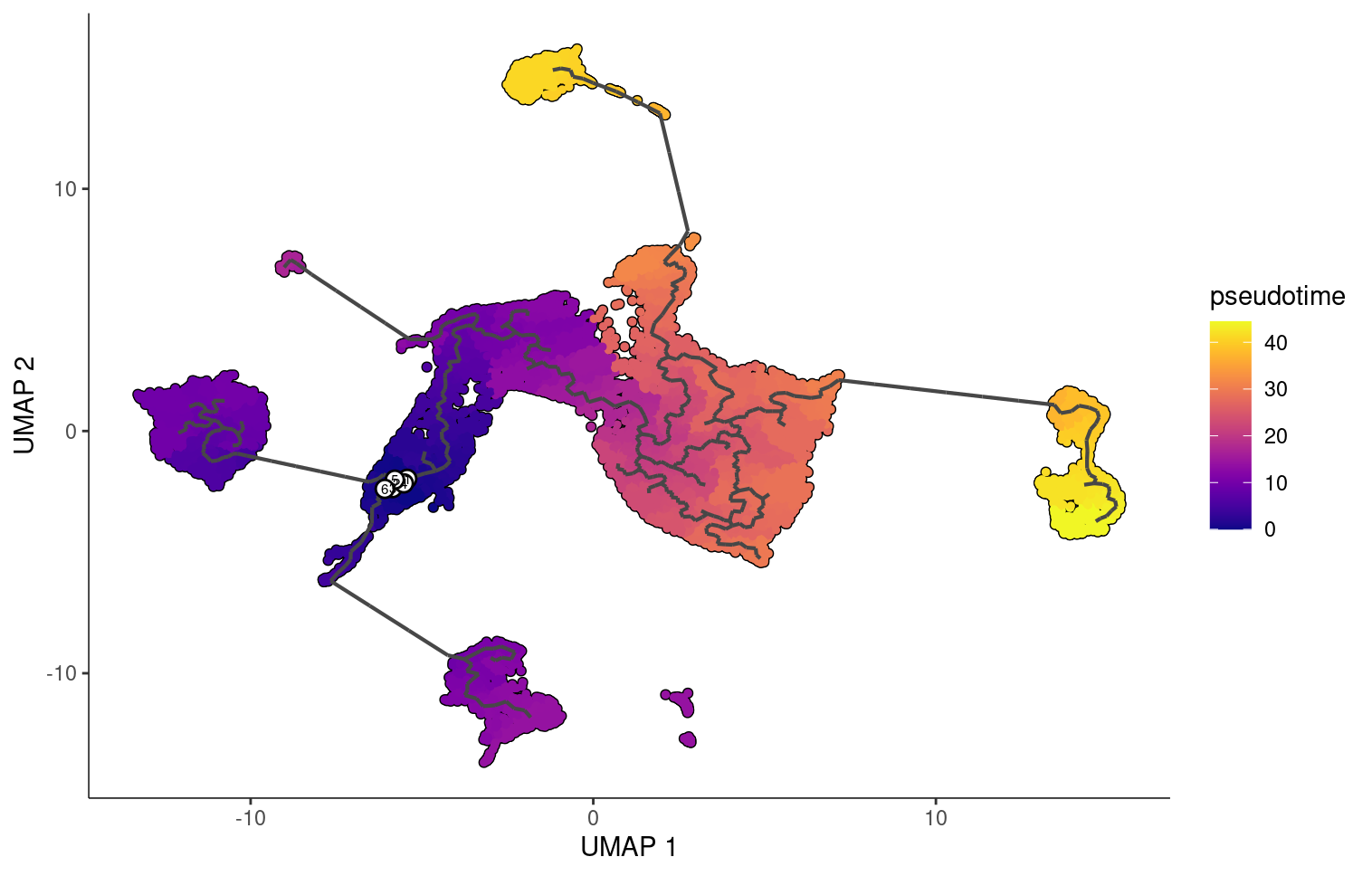
plot_cells(merged_cds, color_cells_by = "pseudotime", label_branch_points = FALSE, label_leaves = FALSE, cell_size = 1)
When we choose a root around where the stem cells are located we see that the fibroblast and epithelial cells end with the higher pseudotime scores.
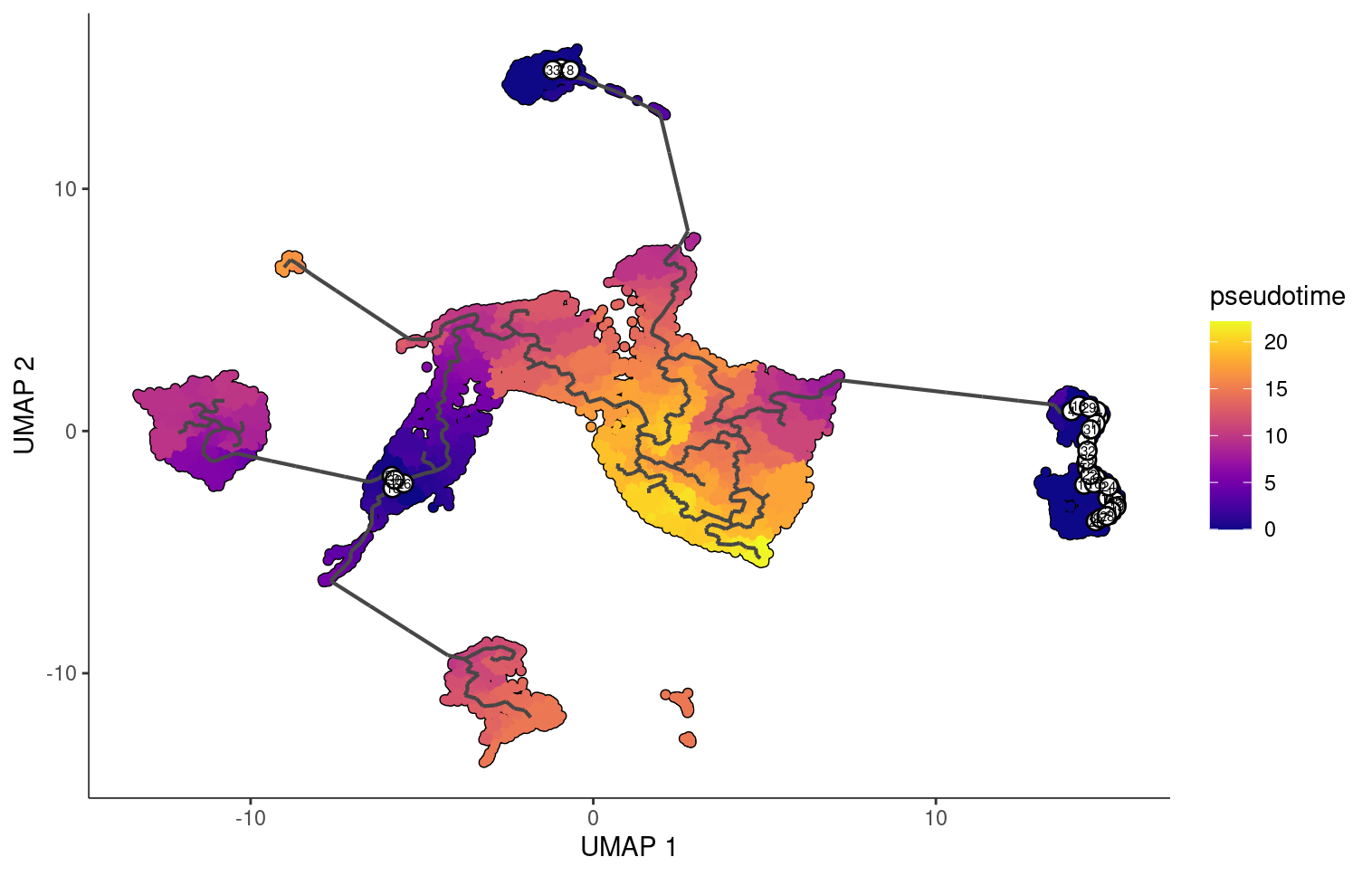
But if we choose are roots to be stem cells, fibroblasts, and epithelial cells, we see that monocle changes the pseudotime orderings accordingly.
We need a significant amount of computational power to run CytoTRACE on all cells so we have run CytoTRACE on a computing cluster and have saved the results to be loaded in and added to our seurat object. Of course, we have to make sure the data is formatted correctly.
# Cytotrace for all cells

# read in the cytotrace scores
merged_cytotrace <- read.table("data/single_cell_rna/reference_files/merged_cytotrace_scores.tsv", sep="\t")
head(merged_cytotrace)


merged_cytotrace_transposed <- t(merged_cytotrace)
colnames(merged_cytotrace_transposed) <- "CytoTRACE"
head(merged_cytotrace_transposed)

rownames(merged_cytotrace_transposed) <- sub("\\.", "-", rownames(merged_cytotrace_transposed))
rownames(merged_cytotrace_transposed)
Now we can add the scores to our seurat object and also create an inverse CytoTRACE score for clarity. So our differentiation score will be 0 for least differentiated (smallest pseudotime) and 1 being most differentiated (biggest pseudotime).
# Add CytoTRACE scores matching on the cell barcodes
merged <- AddMetaData(merged, merged_cytotrace_transposed)
merged[["differentiation_score"]] <- 1 - merged[["CytoTRACE"]]
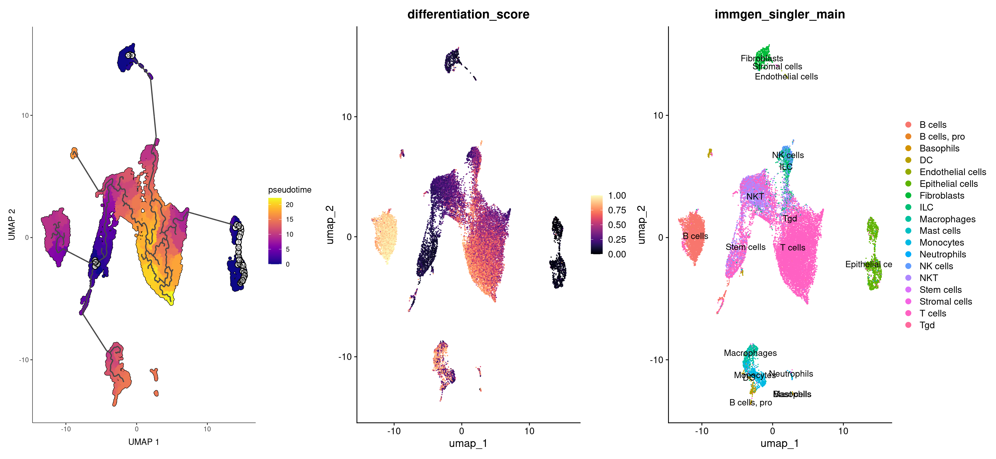
Finally, let’s compare the pseudotime values to our cell types. Do we get the results we want to get? Does Monocle and CytoTRACE agree with each other? What happens if you choose different roots for the Monocle pseudotime?
plot_cells(merged_cds, color_cells_by = "pseudotime", label_branch_points = FALSE, label_leaves =  FALSE, cell_size = 1) +
  (FeaturePlot(merged, features = 'differentiation_score')) +
DimPlot(merged, group.by = 'immgen_singler_main', label = TRUE)
For a final exercise, we can apply the same steps as above to analyze another group of cells: macrophages and monocytes.
highlight = merged$immgen_singler_main =="Macrophages"
highlighted_cells <- WhichCells(merged, expression = immgen_singler_main =="Macrophages")
# Plot the UMAP
DimPlot(merged, reduction = 'umap', group.by = 'orig.ident', cells.highlight = highlighted_cells)


highlight = merged$immgen_singler_main =="Monocytes"
highlighted_cells <- WhichCells(merged, expression = immgen_singler_main =="Monocytes")
# Plot the UMAP
DimPlot(merged, reduction = 'umap', group.by = 'orig.ident', cells.highlight = highlighted_cells)


# grab all cells that are macrophages and monocytes
Idents(merged) <- "immgen_singler_main"
merged_macro_mono_cells <- subset(merged, idents = c("Macrophages", "Monocytes"), invert = FALSE) # 1092

DimPlot(merged_macro_mono_cells, group.by = 'seurat_clusters_res0.8', label = TRUE) +
  DimPlot(merged_macro_mono_cells, group.by = 'immgen_singler_main', label = TRUE)

# grab all cells that are macrophages and monocytes, we can subset by clusters 6 and 14 which seem to contain
Idents(merged) <- "seurat_clusters_res0.8"
merged_macro_mono_cells <- subset(merged, idents = c(6, 14), invert = FALSE) # 1350
DimPlot(merged_macro_mono_cells, group.by = 'seurat_clusters_res0.8', label = TRUE) +
  DimPlot(merged_macro_mono_cells, group.by = 'immgen_singler_main', label = TRUE)

DimPlot(merged_macro_mono_cells, group.by = 'immgen_singler_fine', label = TRUE)
# create a data frame with the counts from our subsetted obect
merged_macro_mono_cells_expression <- data.frame(GetAssayData(merged_macro_mono_cells, layer = "data"))

# pass that dataframe to the CytoTRACE function
merged_macro_mono_cells_cytotrace_scores <- CytoTRACE(merged_macro_mono_cells_expression, ncores = 4)

# Create a dataframe out of the CytoTRACE scores
merged_macro_mono_cells_cytotrace_scores_df <- as.data.frame(merged_macro_mono_cells_cytotrace_scores$CytoTRACE)

# Make the rownames of the cytotraace scores function the cell barcodes and rename the CytoTRACE scores column approproately
rownames(merged_macro_mono_cells_cytotrace_scores_df) <- sub("\\.", "-", rownames(merged_macro_mono_cells_cytotrace_scores_df))
Now we will incorporate our CytoTRACE scores into our Seurat object.
# Add CytoTRACE scores matching on the cell barcodes
merged_macro_mono_cells <- AddMetaData(merged_macro_mono_cells, merged_macro_mono_cells_cytotrace_scores_df)
CytoTRACE assignes the least differentiated cells a score of 1 and the most differentiated cells a score of 0, which is sometimes not inutive. So lets create a inverse CytoTRACE score which we will call our differentiation score.
merged_macro_mono_cells[['differentiation_scores']] <- 1 - merged_macro_mono_cells[['CytoTRACE']]

# Plot the results
DimPlot(merged_macro_mono_cells, group.by = 'seurat_clusters_res0.8', label = TRUE) +
  DimPlot(merged_macro_mono_cells, group.by = 'immgen_singler_main', label = TRUE) +
  FeaturePlot(merged_macro_mono_cells, features = 'differentiation_scores')
Let’s compare our CytoTRACE scores to Monocle3’s trajectory calculations.
cds <- SeuratWrappers::as.cell_data_set(merged_macro_mono_cells)

cds <- cluster_cells(cds)

# View our clusters
plot_cells(cds, show_trajectory_graph = FALSE, color_cells_by = "partition")

cds <- learn_graph(cds, use_partition = FALSE) # graph learned across all partitions
cds <- order_cells(cds) # choose your root(s)
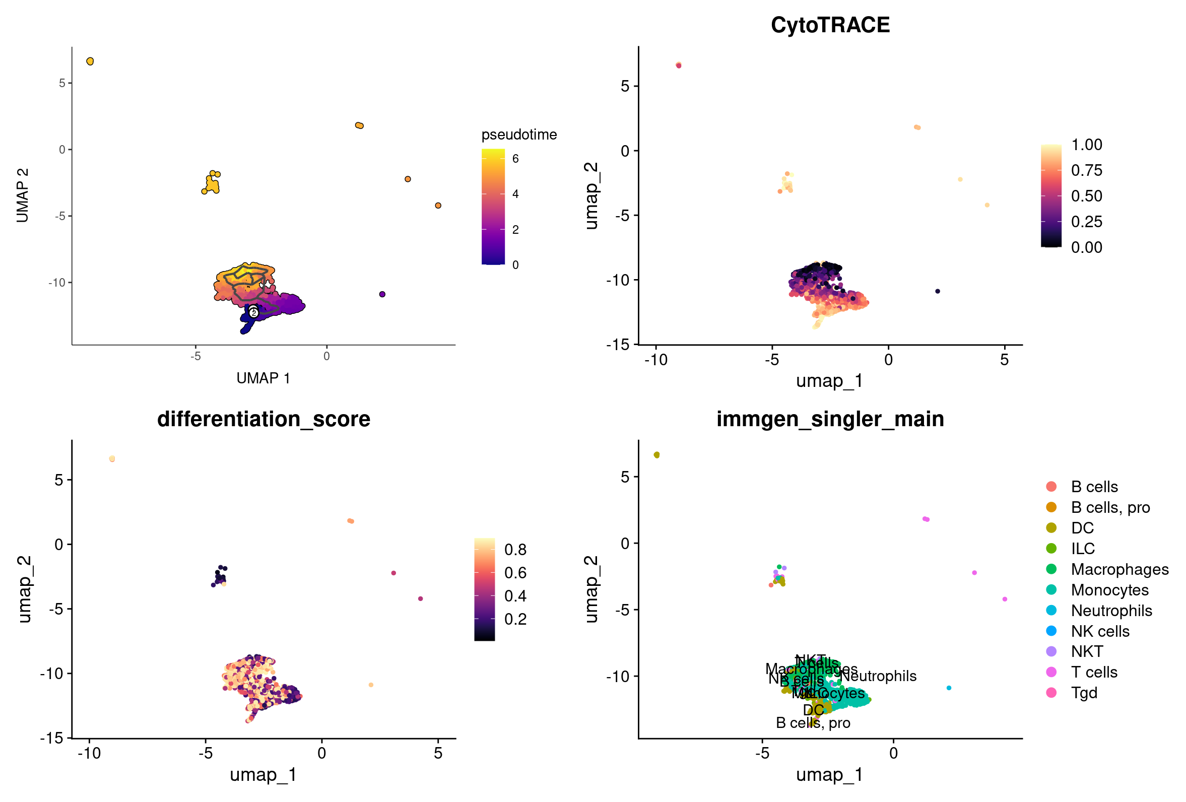
plot_cells(cds, color_cells_by = "pseudotime", label_branch_points = FALSE, label_leaves = FALSE, cell_size = 1)
plot_cells(cds, color_cells_by = "pseudotime", label_branch_points = FALSE, label_leaves =  FALSE, cell_size = 1) +
  (FeaturePlot(merged_macro_mono_cells, features = 'CytoTRACE') + scale_color_viridis(option = 'magma', discrete = FALSE)) +
  (FeaturePlot(merged_macro_mono_cells, features = 'differentiation_score') + scale_color_viridis(option = 'magma', discrete = FALSE)) +
  DimPlot(merged_macro_mono_cells, group.by = 'immgen_singler_main', label = TRUE)
Monocle3 proposes a method to choose a root more precisely in its trajecotry tutorial. It requires you to do the preprocessing steps specific to Monocle3.
merged_cds <- SeuratWrappers::as.cell_data_set(merged)

# Monocle preprocessing steps
merged_cds <- preprocess_cds(merged_cds, num_dim = 50, method = 'PCA')
# merged_cds <- align_cds(merged_cds, alignment_group = "orig.ident") # removes batch effect by fitting its a linear model to the cells
merged_cds <- reduce_dimension(merged_cds, preprocess_method = 'PCA', reduction_method="UMAP") # calculate UMAPs

merged_cds <- cluster_cells(merged_cds)

plot_cells(merged_cds, show_trajectory_graph = FALSE, color_cells_by = "immgen_singler_main")

# monocle will create a trajectory for each partition, but we want all our clusters
# to be on the same trajectory so we will set `use_partition` to FALSE when
# we learn_graph

merged_cds <- learn_graph(merged_cds, use_partition = FALSE) # graph learned across all partitions

# merged_cds <- order_cells(merged_cds)
# Pick a root or multiple roots -- stem cell? or stem cell, fibroblasts, epithelial cells

# a helper function to identify the root principal points:
cell_ids <- which(colData(merged_cds)[, "seurat_clusters_res0.8"] == 5)

closest_vertex <-
  merged_cds@principal_graph_aux[["UMAP"]]$pr_graph_cell_proj_closest_vertex

closest_vertex <- as.matrix(closest_vertex[colnames(merged_cds), ])

root_pr_nodes <-
    igraph::V(principal_graph(merged_cds)[["UMAP"]])$name[as.numeric(names
                                                              (which.max(table(closest_vertex[cell_ids,]))))]
root_pr_nodes

merged_cds <- order_cells(merged_cds, root_pr_nodes=root_pr_nodes)

plot_cells(merged_cds, color_cells_by = "pseudotime", label_branch_points = FALSE, label_leaves =  FALSE, cell_size = 1)
First, we have to export the counts.
merged_mtx <- GetAssayData(merged_epithelial, layer = "counts")
write.csv(merged_mtx, "outdir/merged_epithelial_counts.csv")
Then export the file from posit. In the file window select merged_epithelial_counts.csv. Then go to More -> Export… and click Download.
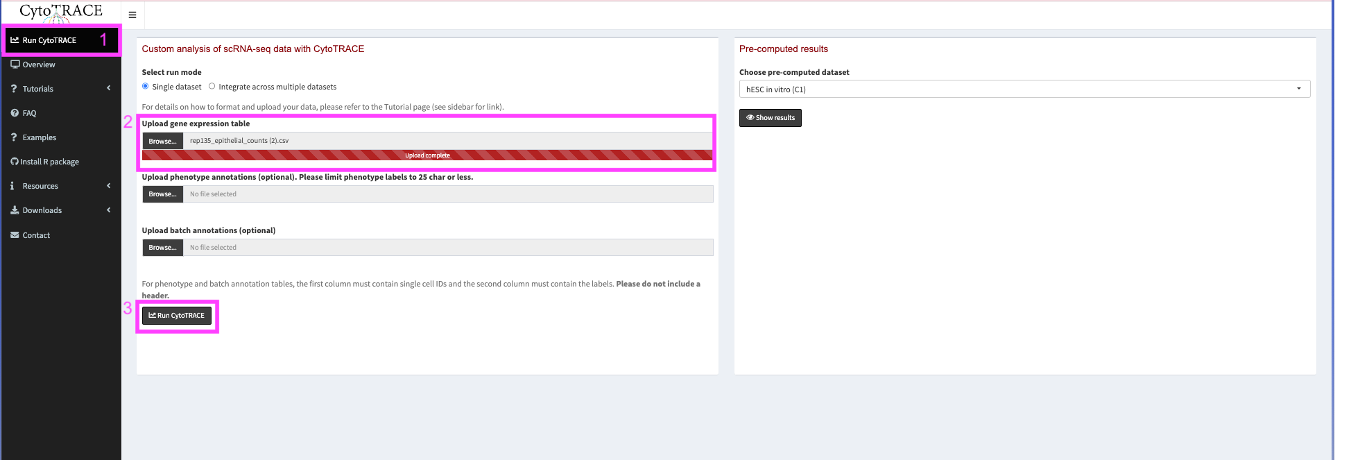
Now we go to https://cytotrace.stanford.edu/. We will navigate to the Run CytoTRACE tab on the left menu bar and upload our downloaded csv in the Upload gene expression table. We will not worry about uploading any other files as of now but if we had a larger dataset we could provide cell type and batch information for our cells.
When uploaded click Run CytoTRACE. This may take a few minutes.
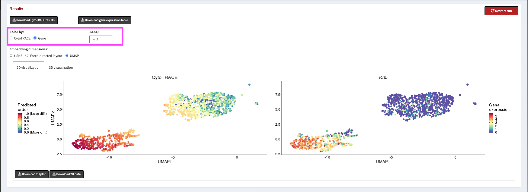
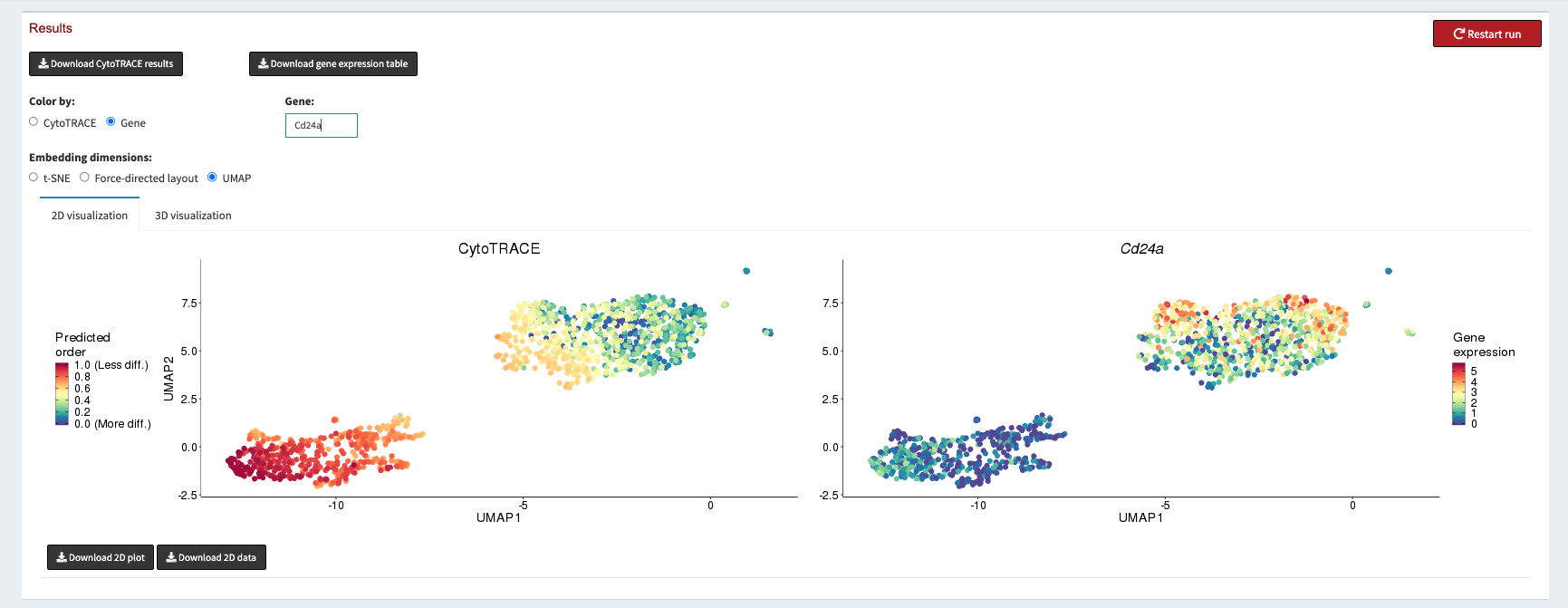
We can then spend some time exploring CytoTRACE scores. For CytoTRACE, warmer colors mean less differentiation, and cooler colors mean more differentiated. We can use the Gene radio button to plot the expression of different marker genes for Basal and Luminal cells.
Once we have verified that the CytoTRACE scores are assigned in a way that corresponds with our biological knowledge we can click the Download CytoTRACE results button at the top left of the page.
We now want to add our CytoTRACE scores to our Seurat object. So we navigate to the Upload button and select our exported CytoTRACE scores from where the file was downloaded. We then read it into R and add the scores to our Seurat object as another column in the meta.data.
cytotrace_scores <- read.table("outdir/CytoTRACE_results.txt", sep="\t") # read in the cytotrace scores

rownames(cytotrace_scores) <- sub("\\.", "-", rownames(cytotrace_scores)) # the barcodes export with a `.` instead of a '-' at the end of the barcode so we have to remedy that before joining the cytotrace scores unto our seurat object

# Add CytoTRACE scores matching on the cell barcodes
merged_epithelial <- AddMetaData(merged_epithelial, cytotrace_scores %>% select("CytoTRACE"))
Now we can plot our basal cell markers, our luminal cell markers, and the CytoTRACE scores together to compare. Since it is a little unintuitive that less differentiated scores are closer to 1 we will also create a differentiation_score which will be an inverse of our CytoTRACE scores so that smaller scores mean less differentiated and larger scores mean more differentiated.
merged_epithelial[['differentiation_scores']] <- 1 - merged_epithelial[['CytoTRACE']] # Let's also reverse out CytoTRACE scores so that high means more differentiated and low means less differentiated

FeaturePlot(object = merged_epithelial, features = c("cell_type_Basal_score1", "cell_type_Luminal_score1", "cytotrace_scores", "differentiation_scores"))